
 Many energy and resource efficiency audits fail to properly address opportunity interdependency in their recommendations, which can greatly reduce the credibility and impact of the audit. This article aims to shed light on this critical aspect of auditing which is also one of the most creative and enjoyable parts of the process.
This post complements an earlier item on the value of involving management in the audit process: “The purpose of a resource efficiency audit”.
The significance of opportunity interdependency
An “opportunity” is simply a description of an action that can be taken to improve resource use. The word “project” is often used interchangeably with “opportunity”, although I feel the latter better encompasses the broader range activities – such a purchasing, project design, behaviour and culture – that can all contribute to better resource use.
The business case for a resource efficiency programme is usually based on a bundle or “portfolio” of many opportunities which have been identified through some form of discovery process, such as an audit or workshop or suggestion scheme or desk study. It is the overall cost and benefits of the portfolio of opportunities that forms the basis for the decision-makers to provide a mandate to take the programme forward.
I believe that there are three steps to a good audit:
- A discovery process which comprehensively quantifies the costs and benefits of individual opportunities; and
- an assessment of how these opportunities interact; and
- the selection of opportunities for inclusion in a portfolio such that the desired business objective can be met and (ideally) opportunities for future improvement are not compromised.
The tricky steps are actually 2 and 3 and it is here that we see many audits fall short. That is not to blame the auditors. Often audits simply do not have enough time and effort behind them so that there is a scramble to find the projects in the first place with little additional time available to synthesise these into a compelling programme of work. In many cases the stated objective of the audit is simply to deliver the first step in the business case process – to provide a list of opportunities – but the recipients of the audit findings are not equipped to complete the additional steps of assessing interactions or creating the optimum portfolio.
The problem is that the benefits of a resource efficiency programme are rarely the simple sum of the individual opportunity costs and benefits of the opportunities proposed. Some projects, for example a lighting reduction project and a water recycling opportunity are genuinely independent in that they are acting on completely different resource streams. In this case the overall costs and benefits are the simple sum of each opportunity. But this is the exception rather than the norm. In most audits we find that multiple opportunities are acting on the same resource streams.
For example, I may have an opportunity to reduce the interior temperature of a building by 3oC which saves, say, 24% on a heating bill and a second opportunity to reduce the heating time from 16 hours to 14 hours which saves 12%. Both of these projects are acting on the same resource stream, the gas I use in my boiler for the purpose of space-heating, so these are said to be compound projects. If I implement both projects the savings will be 33%, less than the simple sum of the savings, which is 36%. This is because the percentage savings compound rather than add together, as can be seen in the table below where the “Start kWh” is reduced to take into account the preceding opportunity savings. Because these projects can be undertaken together they are sometimes called complementary opportunities. We can reduce either heating hours or the space temperature or both.
|
Start kWh |
Saving % |
kWh Saved |
End Kwh |
|
| ↓ Temp 3 Degree |
1,000 |
24% |
240 |
760 |
| ↓ heating hours |
760 |
12% |
91 |
669 |
| Combined Savings |
33% |
331 |
Figure 143 The combined effect of multiple projects impacting the same resource use is not additive but compound. At the end of this post there is a detailed examination of the formulae used to calculate compound savings.
There are other forms of opportunity interdependence that need to be considered when building a business case. Two projects might be mutually exclusive – implementing one prevents the implementation of the other. These projects are referred to as substitute projects, and can be a particular challenge when conducting an audit. This is because most audits are limited by the amount of time and effort available to identify and assess opportunities and the audit team will want to avoid the considerable effort that may be entailed in developing detailed opportunities that will not be taken forward because there is a better alternative. Thus experienced auditors will try to identify substitute projects early on in an assessment, using some high-level screening criteria such as cost or risk, and then focus on the strongest candidate for detailed investigation, reverting to the next strongest alternative if that candidate proves infeasible for some reason.
The opposite effect is seen where a project is contingent on another. Contingency might be mutual, in the sense that either both projects go ahead or none, or single were a second opportunity depends on the first but not vice-versa. Contingent projects often influence the same resource stream so they can also be compound projects. If two or more projects are found to be mutually contingent they are usually merged into a single overarching opportunity for the purposes of the audit in order to reduce some complexity in the subsequent reporting.
The picture of opportunity interactions is further complicated by the fact that some opportunities may influence several resource streams. Thus a project to improve hot water (also known as condensate) return on a steam distribution system will reduce two resources: the boiler-makeup water and the fuel usage. On the other hand a project to eliminate discharges of Volatile Organic Compound (VOC’s) to atmosphere may involve incineration of the waste stream and thus increase fuel usage and CO2 emissions, while decreasing VOC discharge. Many resources are fundamentally and inextricably bound, such as water, wastewater and energy. Reducing water demand reduces the energy used in the distribution, conditioning and treatment of the water. It will also potentially reduce the requirement for chemical inputs and sludge disposal.
These second and third-order impacts can have very significant bearing on the business case for improvement – for example energy is usually a much more expensive input than water, so the business case for reduced water use may be driven by the associated energy costs rather than the water reduction. We have already seen that for many lighting projects it is the reduced parts and labour costs associated with replacing lamps that drives LED investment decisions, rather than just the energy savings.
Portfolio issues
The final recommendations of an audit team usually set out a basket or portfolio of opportunities, not just one single opportunity. The team will therefore need to take into account the interactions and interdependencies of these projects as described above, in order to arrive at the combined business case. If the organisation has a maximum payback or minimum Internal Rate of Return for opportunity approval, then clearly the portfolio of projects needs to meet this hurdle rate, unless there are other overriding non-financial drivers for improvement, such as brand, compliance or ethical objectives.
Assuming that meeting the financial hurdle rate is critical, this then becomes the primary basis for opportunity selection into the portfolio. Where there are mutually exclusive projects or opportunity groups with broadly similar returns, then the most significant added dimension to the selection process tend to be ease of implementation, site acceptance or perceived risk. Thus selecting projects for inclusion into a programme of work or portfolio is by no means a simple as choosing the most cost-effective.
Bundling multiple projects together into a portfolio has a number of advantages:
- The portfolio can include projects which would otherwise fail to meet a financial hurdle rate as they are balanced by projects with a better return;
- Projects can be evaluated sequentially so that cheaper operational demand reduction opportunities are implemented ahead of capital expenditure;
- Programme cost for continuous improvement and management can be more readily justified and allocated;
For example, taking a portfolio approach, the audit team are able to group better and worse performing projects so that in combination they meet the overall financial requirement. Thus if the organisation has a two year or less payback hurdle the portfolio could, in simple terms include a project with a six month payback and a lower cost opportunity with a 36 month payback and achieve an aggregate payback within the two year target. By bundling projects we are able to get approval for opportunities which would not separately meet the approval criteria. This is a very important benefit from systematic audits compared to ad-hoc investigations, as in the ad-hoc approach projects are evaluated independently and so would not normally be approved if above the hurdle rate.
The second benefit of the audit approach is that, assuming the audit team have followed the suggested sequence of investigations set out here, the demand-based opportunities will tend to be prioritised over more expensive equipment or process changes which often require capital. Thus the tendency to “leapfrog” no/low cost opportunities and go straight to equipment upgrades or replacement is avoided.
Displaced Opportunities
Prioritisation of low-cost demand over higher-cost supply solutions can run counter to the objective of achieving the maximum possible resource efficiency – because as demand is reduced by better operation and control, the financial case for the equipment upgrades becomes weaker, potentially pushing the larger capital investments off the table altogether as they no longer meet the hurdle rate in the new more operationally-efficient context. Favouring demand-reduction is logical, cost-effective and will lead to more rapid savings, but can have the unintended result of a lower total improvement.
Opportunity |
|
Opportunity Savings (%) |
Opportunity Cost £ |
Opportunity Saving £ |
Payback (Months) |
|
Single Opportunities |
|||||
| O1: Daylight | £ 205,000 |
15% |
£ 2,937 | £ 30,750 |
1.1 |
| O2: LED | £ 205,000 |
50% |
£ 190,000 | £ 102,500 |
22.2 |
|
Sequential opportunities (best return first) |
|||||
| O1: Daylight | £ 205,000 |
15% |
£ 2,937 | £ 30,750 |
1.1 |
| O2: LED | £ 174,250 |
50% |
£ 190,000 | £ 87,125 |
26.2 |
|
Sequential opportunities (largest first) |
|||||
| O2: LED | £205,000 |
50% |
£ 190,000 | £102,500 |
22.2 |
| O1: Daylight | £102,500 |
15% |
£ 2,937 | £15,375 |
2.3 |
|
Both opportunities combined (Portfolio) |
|||||
| Portfolio | £ 205,000 |
61% |
£ 192,937 | £ 117,875 |
19.6 |
Figure 144 Illustrating the effect that a demand reduction opportunity, O1, has on the investment case for a capital investment opportunity, O2. This is based on a real case for a UK Car Park operator.
The table above shows how demand-side reductions can influence the viability of supply-side measures, to the detriment of the overall savings. This example, based on a real case, involves two opportunities which are complementary: Opportunity O1 is a project to control the car park lighting so that half the lights are switched off when ambient daylight is sufficient high, and requires a modest investment in a daylight sensor to automate the control. Opportunity O2 is based on a quotation for the re-lamping of the car park replacing fluorescent lamps with LED replacements. Given an annual cost of £205,000 on electricity, both opportunities individually meet this organisation’s 2 year or 24-month hurdle rate. Looking at the bottom of the table we can see the combination of both projects into portfolio, with a 19.6 month payback, falls comfortably within the target hurdle rate, so both projects should be approved as a bundle. However a problem arises if opportunity O2 were to be brought forward separately for funding after opportunity O1 had been implemented, as the savings already achieved through the daylight sensor reduce the savings possible through the LED re-lamping, pushing the second opportunity payback to 26.1 months, as shown in red in the table, which above the approval hurdle rate of a 24-month payback. Thus by first implementing a 15% saving on the demand side we have potentially forsaken an initially viable 50% saving on the supply side.
These opportunities which cease to be financially viable as a result of other interventions are called displaced opportunities. Paradoxically the order in which the opportunities are implemented will determine whether they will both meet the necessary return on investment or not. As we can see from the table above, the control opportunity O1 remains financially attractive after the LED change opportunity O2 has been implemented: though the payback has risen from 1.1 months to 2.3 months it still provides a highly attractive return.
Strategies for portfolio design
A judgement that the audit team will need to make in constructing their portfolio of projects is whether early action on some opportunities will displace others. It is advisable to assess the incremental payback from projects as a matter of course when reviewing a portfolio of opportunities. In the event that some opportunities will be displaced, the decision of how to progress is far from clear-cut, and depends largely on the funds available and the organisation’s overall objectives. Here is a summary of the approach that I would take:
- If there is no shortage of funds: i.e. the portfolio of projects will be fully funded so long as it meets the required hurdle rate, I will incorporate as many projects as I can in the portfolio which maximise the improvement and still ensure that the portfolio as a whole meets the required return. In this case both opportunities O2 and O1 would get approved as part of the overall portfolio of opportunities and the order of implementation is not relevant.
- If there is a shortage of funds or a fixed target for improvement, which means that some projects within the hurdle rate will not be funded, I will tend to try to include any projects that could be displaced in the initial list of recommendations to be implemented. This may mean that these opportunities are given preference over some opportunities with better return, but the latter can still be taken forward at a later date knowing that they will still meet the hurdle rate. In this case I would tend to recommend opportunity O2 over O1 and explain to the decision-maker why a lower return on investment at the outset makes more sense in the long-run.
- An alternative is to treat the opportunity causing the displacement and the potentially displaced opportunity as if they are mutually contingent and merge them into one single new opportunity. Thus I could have an opportunity O3 “Car Park Lighting Improvements”, which is the combination of opportunities O1 and O2, with a payback of 19.6 months. However I would need to be careful that this project will pass the approval hurdle else I risk throwing out the “no brainer” opportunity O1 out of the mix of projects taken forward.
We can see that bundling projects together into a portfolio that meets short term objectives while maintaining the capacity for further longer-term improvements can be quite complex. The process of developing the right portfolio for a given situation is immensely creative. There will be aspects of confidence, risk, ease of implementation, repeatability and the preferences of decision-makers to consider. This project assembly process is possibly the most exciting and interesting part of the audit. It is as if the individual opportunities are bricks from which we have to construct the right structure to start the organisation towards their desired destination – this is “architecture” of the highest and most satisfying form.
Far too often the findings of energy and resource efficiency audits are summarised in a list of projects with their individual return on investment calculated as if they are all independent. This failure to properly assess project interdependency leads to some severe problems:
- It leads to an overstatement of potential, and unrealistic expectations;
- It undermines the credibility of the audit findings which severely impacts on the ability to gain management commitment to proceed (see “Why certainty matters”);
- It leads to cherry picking of projects and undermines the concept of continuous improvement and a systematic approach (see “the Hare and the Tortoise”);
- Which in turn leads to displacement of opportunities and overall net reduction in the improvements made.
Thus the process of assessing opportunity interactions and gathering the best opportunities for a particular organisation’s needs is essential in gaining a Mandate for a resource efficiency program.
A Classification of opportunity interdependencies
Compound: these are opportunities that act on the same resource streams and so have an effect on each other. Compound opportunities can be further categorised: |
||
| Complementary: opportunities that can be undertaken separately. Thus I could implement either opportunity A or opportunity B in any order, so A and B are complementary. Contingent: opportunities which are mutually dependent. For example where project B can only be implemented if we carry out project A first, B is said to be contingent on A. Contingent project can be further classified as: |
||
| Mutually contingent: where both project A and B need to be implemented to deliver the improvement, they can be said to be mutually contingent. Singly contingent: where B depends on A, but not vice-versa, B is singly contingent on A. |
||
| Substitute: opportunities which are mutually exclusive. If I undertake project A then project B is no longer feasible (or vice-versa). Thus projects A and B are substitutes or A is a substitute for B.Rarely, substitute opportunities can arise in projects which affect different resource streams – for example we could implement a CHP plant generate electricity on-site or a waste-water treatment plant to reduce effluent, but either project would use all the available free land so rather than being independent opportunities by virtue of impacting different resource streams, they are mutually exclusive or substitutes. |
||
| Finally any type of project can also be Displaced. This occurs when a preceding opportunity leads to an opportunity becoming infeasible for technical or financial reasons. This is different from substitute opportunities as the order of implementation is what determines the feasibility. Thus project A may be feasible if project B has been implemented first but project B may be infeasible if project A has already been implemented. Thus B is displaced by A (but not A by B). Displacement is usually due to financial feasibility issues rather than technical issues. The example above illustrates how a decline in the starting resource requirement due to earlier action invalidates the business case for a subsequent project. A more common example of displacement of projects across resource streams occurs in the scenario where an organisation has a limited amount of capital to spend. There may be a large number of projects that meet a particular financial return, but once the capital is allocated the remaining projects requiring capital are effectively displaced. | ||
Calculating saving for compound opportunities
Calculating the effective saving rate from multiple projects acting on the same resource stream involves compounding the individual project savings rate.
Let’s take a simple example to illustrate the process of compounding, which we briefly described earlier. In this example we have an opportunity to reduce the interior temperature of an office by 3oC which saves 24% on a heating bill and a second project to reduce the heating time from 16 hours to 14 hours which saves 12%. Both of these projects are acting on the same resource stream, the gas I use in my boiler, so these are compound projects.
If I imagine my initial weekly kWh of gas usage is 1000 then if I implement the first project I will reduce this by 24% leading to a weekly usage of 760 kWh, as shown in the table below. When it comes to considering the second project, which delivers 12% savings, it is important to note these savings are calculated against the reduced usage of 760 kWh after Project 1, not the original 1000 kWh. Taking this into account I can see that Project 2 will save 12% of 760 kWh, or 91.2 kWh, leaving me with a final gas usage of 668.8 kWh. This is 331.2 kWh less than I initially used which gives both projects a combined saving of 33%, not the 36% that the sum of the two savings rates would have suggested.
|
Start kWh |
Saving r |
Saved kWh |
End kWh |
|
|
P1: ↓ Temp 3 Degree |
1,000.00 (S1) |
24% (0.24 r1) |
240.00 |
760.00 (E1) |
|
P2: ↓ heating hours |
760.00 (S2) |
12% (0.12 r2) |
91.20 |
668.80 (E2) |
|
Combined Savings |
33.12% |
331.20 |
Figure 146 The savings from two projects acting on the same resource stream are compounded as shown in the table above. Notation refers to the formulae in the text below.
Turning this into an algebraic expression let us define S1 as our starting quantity of resource used (1000 kWh in the example above) and r1 is the savings rate for the first project (i.e. 24% expressed as 0.24) and E1 is the end quantity of resource after applying the savings rate for the first project (760 in the example above).
For just one project the end units are determined by the formula:
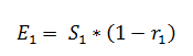
This assumes the conventional approach that savings are expressed as a positive number, thus 10% savings is expressed as 0.1. If savings are expressed as a negative number the minus sign above becomes a plus.
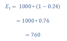
Going back to our simple example we can see that the end consumption following our first project with starting energy use of 1000 kWh and savings rate of 24% (i.e. 0.24) will be 760 kWh, as follows:
We can generalise this first equation for multiple projects, 1 to n, in effect decreasing the initial consumption S1 by the percentage savings rate of each project one by one until project n where we reach En:
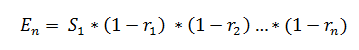
Again substituting in our example numbers we can see that for the two projects above:
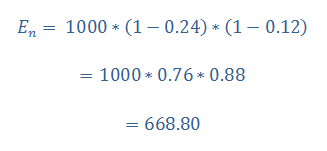
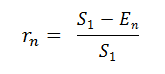
In many cases it is actually more useful to have a figure for the total savings percentage from the basket of projects. OK so in the example above we have saved S1 – En kWh.
To get the effective savings rate for both projects combined, we do the usual percentage calculation:
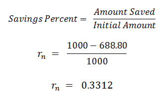
If we want to express our savings in percentage terms we multiply 0.3312 by 100 to give us 33.12% as a percentage savings rate from the combination of both projects.
In algebraic terms the formula we have used above is:
Since we already have an expression for En we can substitute this into our formula to above:
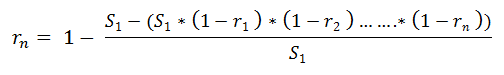
If we then simplify by eliminating the starting units S1, we get an equation to calculate the compound savings rate of n projects acting on the same resource stream:
![]()
For a printable pdf version of this post please click here, as most browsers do not accurately position the formulae centrally.
For more ideas and challenges check out all the posts on this site.
Learn what an effective resource efficiency framework looks like.
Read reviews of books on the theme of change.
Or learn how SustainSuccess services can drive improvement in your organisation.


0 Comments